When training machine learning algorithms, complex models frequently fit training data too closely, learning random noise rather than true structural patterns. This manifests as high variance and poor generalization on unseen validation data.
To prevent overfitting without sacrificing expressive capacity, machine learning relies on regularization—a mathematical technique that penalizes overly large or complex model parameters.
The two foundational techniques are L1 Regularization (Lasso) and L2 Regularization (Ridge). Understanding how their penalty mechanics differ is critical for feature selection, model interpretability, and robust performance.
1. The Cost of Complexity: Why Regularize?
In standard linear models (like Ordinary Least Squares regression), the algorithm minimizes a loss function—such as Mean Squared Error (MSE):
$$\text{Loss}{\text{standard}} = \sum{i=1}^{n} (y_i - \hat{y}_i)^2$$
When features are correlated, redundant, or outnumber training samples ($p > n$), the optimization algorithm often compensates by assigning massive, opposing positive and negative weights ($\mathbf{w}$) to features. While this yields near-zero training loss, tiny fluctuations in test inputs cause erratic, swinging predictions.
Regularization addresses this by augmenting the loss function with an explicit complexity penalty:
$$\text{Objective Loss} = \text{Data Loss (MSE)} + \lambda \cdot \Omega(\mathbf{w})$$
The regularization parameter $\lambda$ (or $\alpha$) acts as a tuning knob:
- $\lambda = 0$: Standard unpenalized model (vulnerable to overfitting).
- High $\lambda$: Harsh parameter shrinkage (drives model toward high bias/underfitting).
- Optimal $\lambda$: Balanced complexity curve that minimizes test error.
2. L1 Regularization (Lasso Regression)
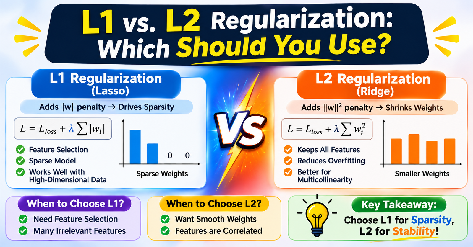
L1 regularization (Least Absolute Shrinkage and Selection Operator) penalizes the model based on the sum of the absolute values of the feature coefficients.
Mathematical Formulation
$$\text{Loss}{L1} = \text{MSE} + \lambda \sum{j=1}^{p} \vert{}w_j\vert{}$$
Key Characteristic: Feature Sparsity
The primary distinguishing feature of L1 is that it drives unimportant feature coefficients completely to zero.
Because coefficients can hit exactly zero, Lasso performs automatic feature selection. If you feed a dataset with 500 features into an L1-regularized model, it may zero out 460 of them, leaving a sparse, highly interpretable model that relies only on the 40 most informative predictors.
When to Use L1:
- You have high-dimensional datasets with many sparse or irrelevant features.
- Model interpretability and compact storage are top priorities.
- You want the model to isolate and retain only the most critical subset of predictors.
3. L2 Regularization (Ridge Regression)
L2 regularization (Ridge regression / Tikhonov regularization) penalizes the model based on the sum of the squared values of the feature coefficients.
Mathematical Formulation
$$\text{Loss}{L2} = \text{MSE} + \lambda \sum{j=1}^{p} w_j^2$$
Key Characteristic: Proportional Weight Shrinkage
L2 penalizes large weights exponentially harder than small weights. As a result, it pulls all coefficients toward zero, shrinking their magnitudes smoothly and evenly.
Crucially, L2 never forces coefficients to absolute zero (unless $\lambda \to \infty$). All original features remain in the model, but their influence is damped down so that no single feature dominates predictions.
When to Use L2:
- You have many collinear or highly correlated features (L2 distributes weight evenly across correlated groups, whereas L1 arbitrarily picks one).
- Most features are believed to hold true underlying signal, meaning you want shrinkage rather than feature elimination.
- Baseline predictive accuracy is prioritized over extreme feature sparsity.
4. Geometric Intuition: Why L1 Yields Sparsity
The mathematical reason L1 forces weights to zero while L2 only shrinks them lies in the geometric shape of their constraint regions:
       L1 (Lasso): Diamond Constraint         L2 (Ridge): Circular Constraint
                   w2                                     w2
                   ^                                      ^
                   |                                      |
                 / | \                                  .---.
                /  |  \                                /     \
               /   |   \                              |   o---|--> w1
       --------+---+---+--------> w1          --------+---+---+--------> w1
                \  |   /                               \     /
                 \ |  /                                 '---'
                  \|/                                     |
                   |                                      |
     (Corners touch coordinate axes)           (Smooth boundary, no sharp corners)