Every supervised machine learning workflow centers around one fundamental challenge: training a model that performs accurately not just on the data it has already seen, but on new, unseen test data.
When a predictive algorithm fails to generalize, the problem almost always traces back to a tension known as the bias-variance tradeoff. Striking the right balance between these two sources of error is one of the most critical steps in building robust machine learning systems.
1. What Is Bias?
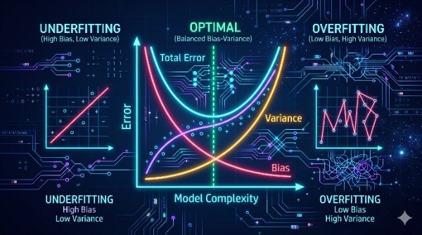
Bias measures how far off a model's average predictions are from the true underlying values across different training sets. It stems from simplistic or erroneous assumptions made by the learning algorithm.
- High Bias (Underfitting): Occurs when an algorithm makes overly rigid assumptions about the data distribution. Because the model lacks sufficient capacity or feature representation, it fails to capture the true underlying signal.
- Symptoms: High error on the training dataset and equally high error on validation/test sets.
- Typical Examples: Fitting a simple straight linear regression line to data governed by a steep quadratic or exponential curve.
2. What Is Variance?
Variance measures how much a model’s predictions fluctuate when trained on different subsets of data drawn from the same underlying distribution.
- High Variance (Overfitting): Occurs when an algorithm is excessively flexible or complex. Instead of learning only the true structural patterns, the model fits the random noise, outliers, and quirks unique to its specific training sample.
- Symptoms: Extremely low (or near-zero) error on training data, coupled with a dramatic spike in error when evaluated on unseen validation or test data.
- Typical Examples: Unconstrained decision trees with deep splits, high-degree polynomial regressions ($d \ge 15$), or over-parameterized neural networks trained without regularization.
3. The Mathematical Decomposition of Error
In supervised learning settings (such as mean squared error regression), the expected test error for a given input $x$ decomposes cleanly into three distinct components:
$$\text{Expected Error} = \text{Bias}^2 + \text{Variance} + \sigma^2$$
Where:
- $\text{Bias}^2$: The error introduced by approximating a complex real-world phenomenon with a simplified model family.
- $\text{Variance}$: The error introduced by the model's sensitivity to small fluctuations in the training dataset.
- $\sigma^2$ (Irreducible Error): The fundamental noise floor present within the data itself (due to unmeasured features, measurement errors, or inherent randomness). Even a theoretically perfect model cannot eliminate irreducible error.
4. The Tradeoff Dynamic
Model capacity directly dictates where an algorithm lands along the spectrum: