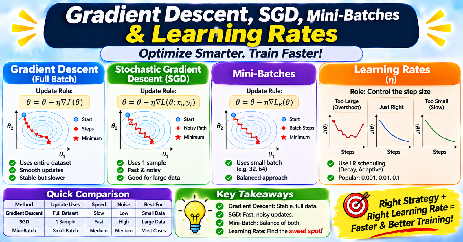
Every machine learning model—from simple linear regression to multi-billion parameter neural networks—learns by minimizing an objective loss function $J(\theta)$. The mathematical mechanism that drives this parameter tuning is Gradient Descent.
Understanding how gradient descent navigates high-dimensional loss landscapes, how batch sizes alter convergence paths, and how the learning rate controls stability is central to training modern machine learning models.
1. The Core Intuition: Walking Downhill
Imagine being stranded on a fog-covered mountain at night with zero visibility. To find the valley floor (the point of minimum error), you feel the slope of the ground beneath your feet and take a step in the steepest downward direction.
In mathematics, the gradient $\nabla_\theta J(\theta)$ is a vector containing the partial derivatives of the loss function with respect to every model parameter $\theta$:
$$\nabla_\theta J(\theta) = \left[ \frac{\partial J}{\partial \theta_1}, \frac{\partial J}{\partial \theta_2}, \dots, \frac{\partial J}{\partial \theta_d} \right]^T$$
Because the gradient points in the direction of steepest ascent (maximum increase), we step in the opposite direction:
$$\theta_{t+1} = \theta_t - \eta \cdot \nabla_\theta J(\theta_t)$$
Where:
- $\theta_t$: Current model weights at step $t$.
- $\eta$ (eta): The learning rate (step size).
- $\nabla_\theta J(\theta_t)$: Steepest slope of the loss function.
2. The Three Variants of Gradient Descent
The primary distinction among gradient descent variants is the amount of training data used to compute each individual gradient step.
Batch GD (All Data)              SGD (1 Sample)               Mini-Batch GD (32-256 Samples)
       \                                |                             \
        \  (Smooth, direct)             | (Noisy, erratic)             \  (Balanced, fast)
         \                             / \                              \
          v                           v   \                              v
       [Minimum]                     [Minimum]                        [Minimum]