In real-world data science, the vast majority of collected data arrives without neat ground-truth labels. Manually annotating millions of records is expensive, slow, and often impossible.
To extract actionable intelligence from unlabeled data, machine learning relies on Unsupervised Learning. The two foundational workhorses in this domain are:
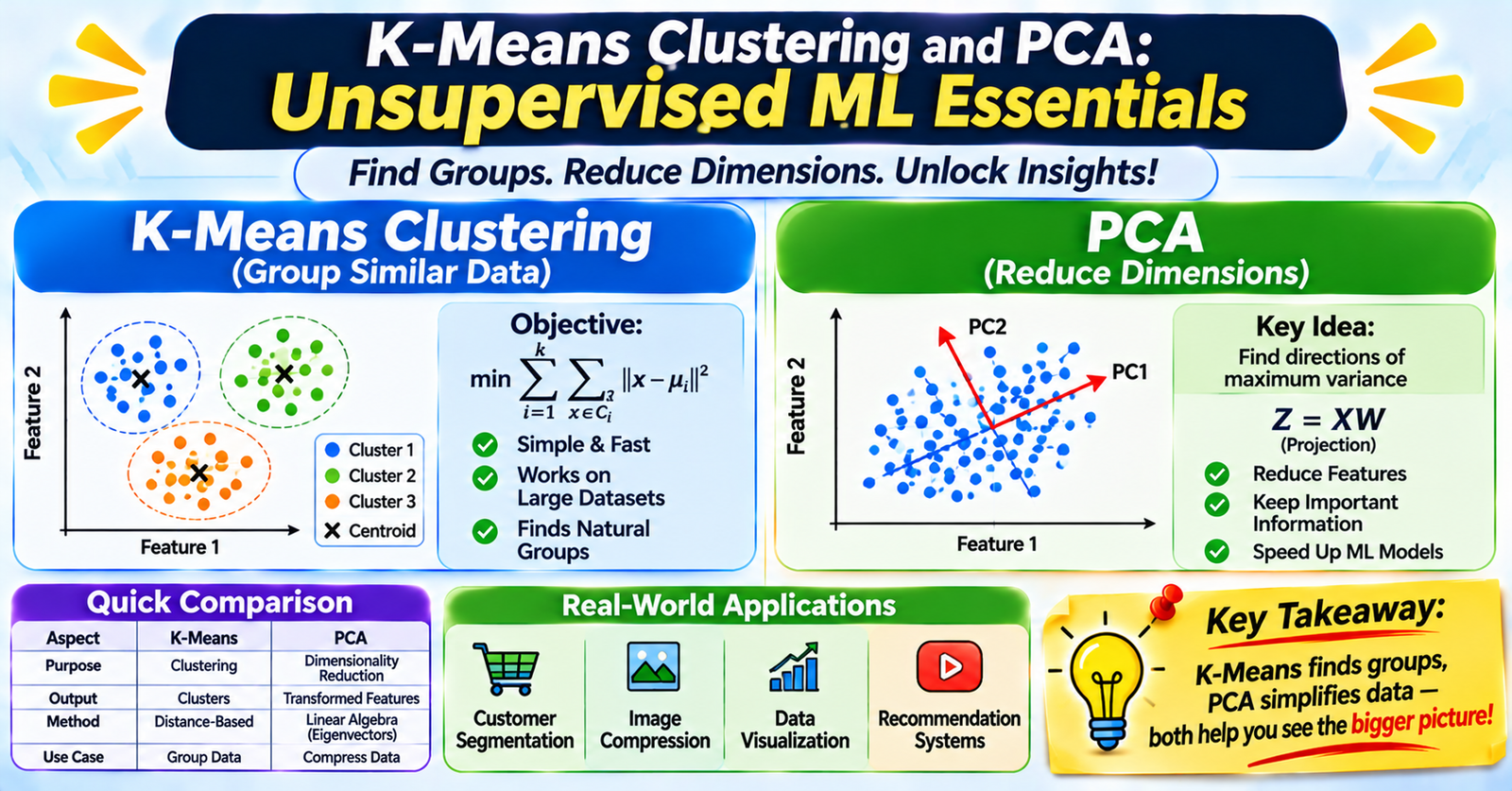
- K-Means Clustering: Discovers natural, discrete groupings and segments across unlabeled data points.
- Principal Component Analysis (PCA): Compresses high-dimensional feature spaces into compact representations while retaining as much informative variance as possible.
Understanding both techniques—and how they complement each other—is essential for exploratory data analysis, data compression, and customer segmentation.
1. K-Means Clustering: Finding Natural Clusters
K-Means is a centroid-based, iterative partitioning algorithm. It groups $N$ observations into $K$ distinct, non-overlapping clusters where each point belongs to the cluster with the nearest mean (centroid).
How the Algorithm Works (Lloyd's Algorithm)
- Initialization: Choose $K$ (number of clusters) and randomly place $K$ initial cluster centroids $\mu_1, \mu_2, \dots, \mu_K$ across the feature space.
- Assignment Step: Assign each data point $x_i$ to its closest centroid using squared Euclidean distance: $$c^{(i)} = \arg\min_j \Vert{}x_i - \mu_j\Vert{}^2$$
- Update Step: Recalculate each centroid position by computing the arithmetic mean of all data points currently assigned to that cluster: $$\mu_j = \frac{1}{\vert{}S_j\vert{}} \sum_{i \in S_j} x_i$$
- Convergence: Repeat the assignment and update steps until centroids stop shifting (or a maximum iteration threshold is met).
The Objective Function (Inertia)
K-Means minimizes the Within-Cluster Sum of Squares (WCSS), also known as Inertia:
$$\text{WCSS} = \sum_{j=1}^{K} \sum_{i \in S_j} \Vert{}x_i - \mu_j\Vert{}^2$$
Selecting Optimal $K$
- The Elbow Method: Plot WCSS against candidate values of $K$. Look for the distinct "elbow" point where adding more clusters yields diminishing returns in variance reduction.
- Silhouette Analysis: Measures how similar a point is to its own cluster compared to neighboring clusters. Scores range from $-1$ (poorly assigned) to $+1$ (dense, distinct cluster separation).
Crucial Caveats with K-Means
- K-Means++ Initialization: Standard random initialization often traps the model in poor local minima. K-Means++ selects initial centroids spaced far apart from each other, ensuring faster and more reliable convergence.
- Spherical & Variance Assumption: K-Means assumes clusters are roughly spherical, similarly sized, and have comparable densities. It struggles with elongated, concentric, or irregular cluster geometries (where density-based algorithms like DBSCAN excel).
- Mandatory Feature Scaling: Because distance computations rely on Euclidean metrics, unscaled features with large numerical magnitudes will overwhelm smaller features. Always standardize features with zero mean and unit variance.
2. Principal Component Analysis (PCA): Dimensionality Reduction
As datasets expand to hundreds or thousands of features, models encounter the Curse of Dimensionality: feature space expands exponentially, distance metrics lose contrast, and models overfit.
Principal Component Analysis (PCA) is an orthogonal linear transformation that maps high-dimensional data into a lower-dimensional coordinate space without requiring target labels.
Mathematical Objective
PCA constructs new uncorrelated variables called Principal Components (PCs). Each PC is a linear combination of original features:
- PC1 (First Principal Component): The directional vector along which the data exhibits the maximum variance.
- PC2 (Second Principal Component): The direction orthogonal (perpendicular) to PC1 that captures the highest remaining variance.
- Subsequent components continue capturing the maximum orthogonal variance.
How PCA Is Computed
- Standardize the Data: Ensure every feature has $\mu = 0$ and $\sigma = 1$.
- Compute Covariance Matrix ($\Sigma$): Calculates linear relationships between all feature pairs ($p \times p$ matrix): $$\Sigma = \frac{1}{n-1} X^T X$$
- Eigendecomposition or SVD: Calculate the Eigenvectors (which define the principal axes directions) and Eigenvalues (which define the variance magnitude explained by each axis).
- Project Data: Sort eigenvectors by descending eigenvalues, select the top $k$ components, and project original data into the lower-dimensional $k$-subspace.
Explained Variance Ratio
To decide how many dimensions to keep, plot the cumulative Explained Variance Ratio:
$$\text{Explained Variance} = \frac{\lambda_j}{\sum_{i=1}^p \lambda_i}$$
A standard rule of thumb is to retain enough components to preserve $90\%$ to $95\%$ of the total original variance.
3. Head-to-Head Comparison
| Attribute | K-Means Clustering | Principal Component Analysis (PCA) |
|---|---|---|
| Primary Goal | Group similar samples into $K$ clusters | Reduce feature dimensions ($p \to k$) |
| Output Type | Discrete cluster assignments ($0, 1, \dots, K-1$) | Continuous projected coordinate coordinates |
| Data Reduction Axis | Partitions along rows (instances) | Compresses along columns (features) |
| Underlying Math | Voronoi tessellation, Euclidean distance | Covariance matrix eigendecomposition, SVD |
| Feature Scaling | Mandatory (Euclidean metric) | Mandatory (Variance sensitive) |
| Interpretability | Moderate (interpreting centroid profiles) | Low (features are combined into linear mixtures) |
4. Combining PCA and K-Means in Practice
PCA and K-Means form a powerful two-stage pipeline:
High-Dimensional Data (e.g., 200 Features)
                  │
                  ▼
   [ Standardize Features (Z-Score) ]
                  │
                  ▼
       [ PCA Reduction (e.g., 200 -> 10 PCs) ]
       - Eliminates multicollinearity
       - Removes high-frequency noise
       - Accelerates distance calculations
                  │
                  ▼
      [ K-Means Clustering on Reduced PCs ]
                  │
                  ▼
Clean, Distinct Customer Segments / Visualizations