Linear regression and logistic regression are the two foundational building blocks of supervised machine learning. While they share similar linear mathematical cores, they solve fundamentally different problems: one predicts continuous quantities, while the other predicts discrete probabilities and categories.
Confusing their mechanics or applying linear regression to classification tasks is a classic practitioner mistake. Here is how both algorithms work, how their loss formulations differ, and how to decide which to deploy.
1. Linear Regression: Predicting Continuous Quantities
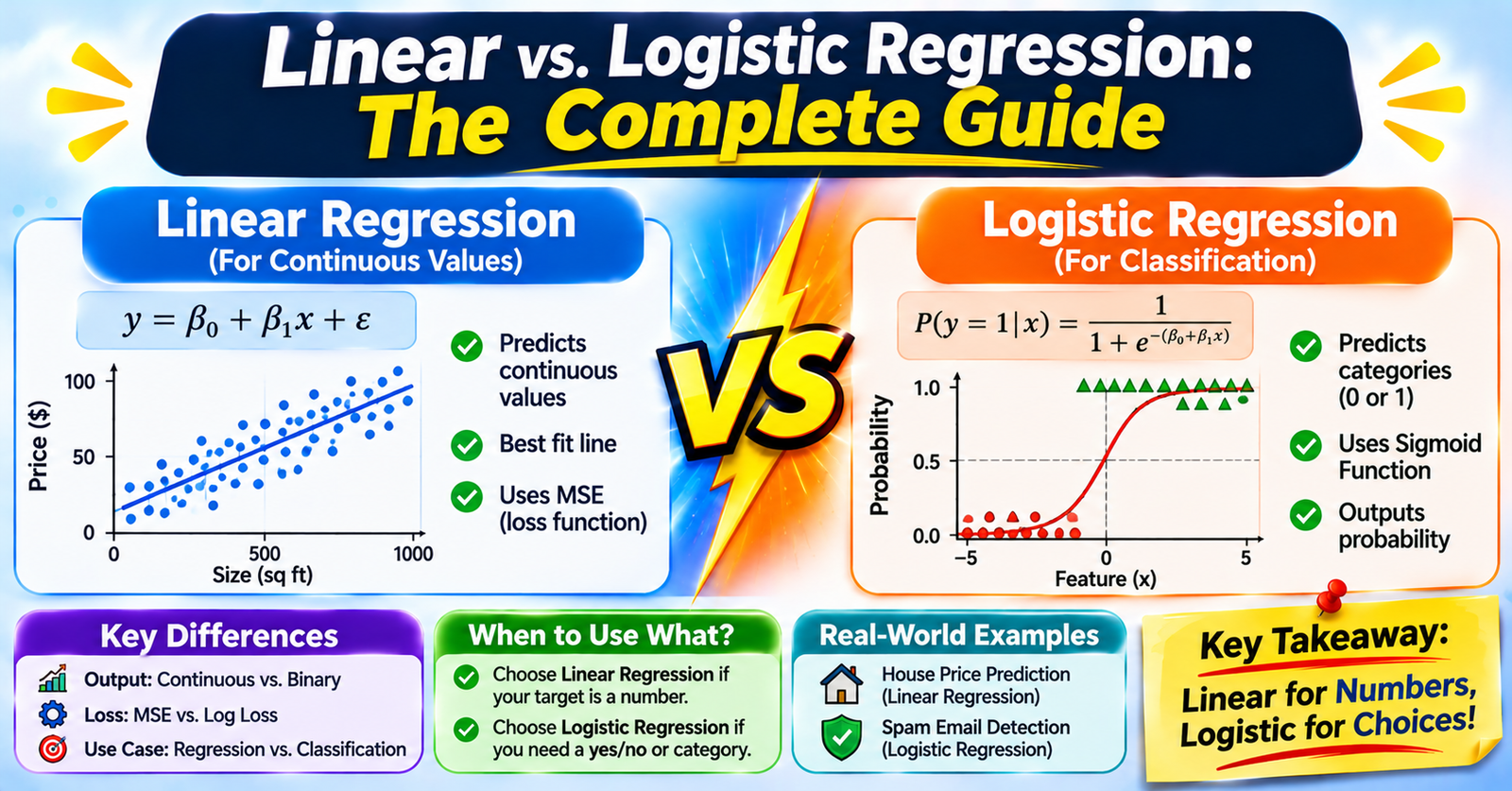
Linear regression models the relationship between one or more independent feature inputs ($X$) and a continuous target variable ($y \in \mathbb{R}$).
Mathematical Formulation
The algorithm assumes the target is a linear combination of input features plus an intercept (bias) term:
$$\hat{y} = w_0 + w_1 x_1 + w_2 x_2 + \dots + w_p x_p = \mathbf{w}^T \mathbf{x}$$
- Output: Any continuous real number from $-\infty$ to $+\infty$.
- Objective: Find the line, plane, or hyperplane that minimizes the total vertical distance between actual data points and predicted values.
Loss Function: Mean Squared Error (MSE)
Linear regression optimizes parameters by minimizing the sum of squared residuals via Ordinary Least Squares (OLS) or gradient descent:
$$J(\mathbf{w}) = \frac{1}{n} \sum_{i=1}^{n} (y_i - \mathbf{w}^T \mathbf{x}_i)^2$$
This loss surface is strictly convex (a smooth bowl shape), guaranteeing a single global minimum without local minima traps.
Common Applications
- Real estate price estimation.
- Demand and revenue forecasting.
- Temperature and energy load prediction.
2. Logistic Regression: Predicting Probabilities and Classes
Despite containing "regression" in its name, logistic regression is a classification algorithm. It models the probability that a given observation belongs to a particular binary class ($y \in \{0, 1\}$).
The Sigmoid Activation
If you fit a standard straight line to binary targets (0 and 1), the line will predict nonsensical values like $-0.4$ or $+1.8$.
Logistic regression solves this by taking the raw linear score ($z = \mathbf{w}^T \mathbf{x}$) and passing it through the logistic sigmoid function $\sigma(z)$, compressing the output strictly into a valid probability range between $0$ and $1$:
$$\sigma(z) = \frac{1}{1 + e^{-z}}$$
$$\hat{p} = P(Y = 1 \mid \mathbf{x}) = \frac{1}{1 + e^{-\mathbf{w}^T \mathbf{x}}}$$
  Probability P(Y=1)
        ^
    1.0 |                              .--------
        |                            .'
        |                          .'
    0.5 | - - - - - - - - - - - - +  (Decision Threshold)
        |                       .'
        |                     .'
    0.0 | --------'----------+------------------->
                             0.0                  z = w^T x