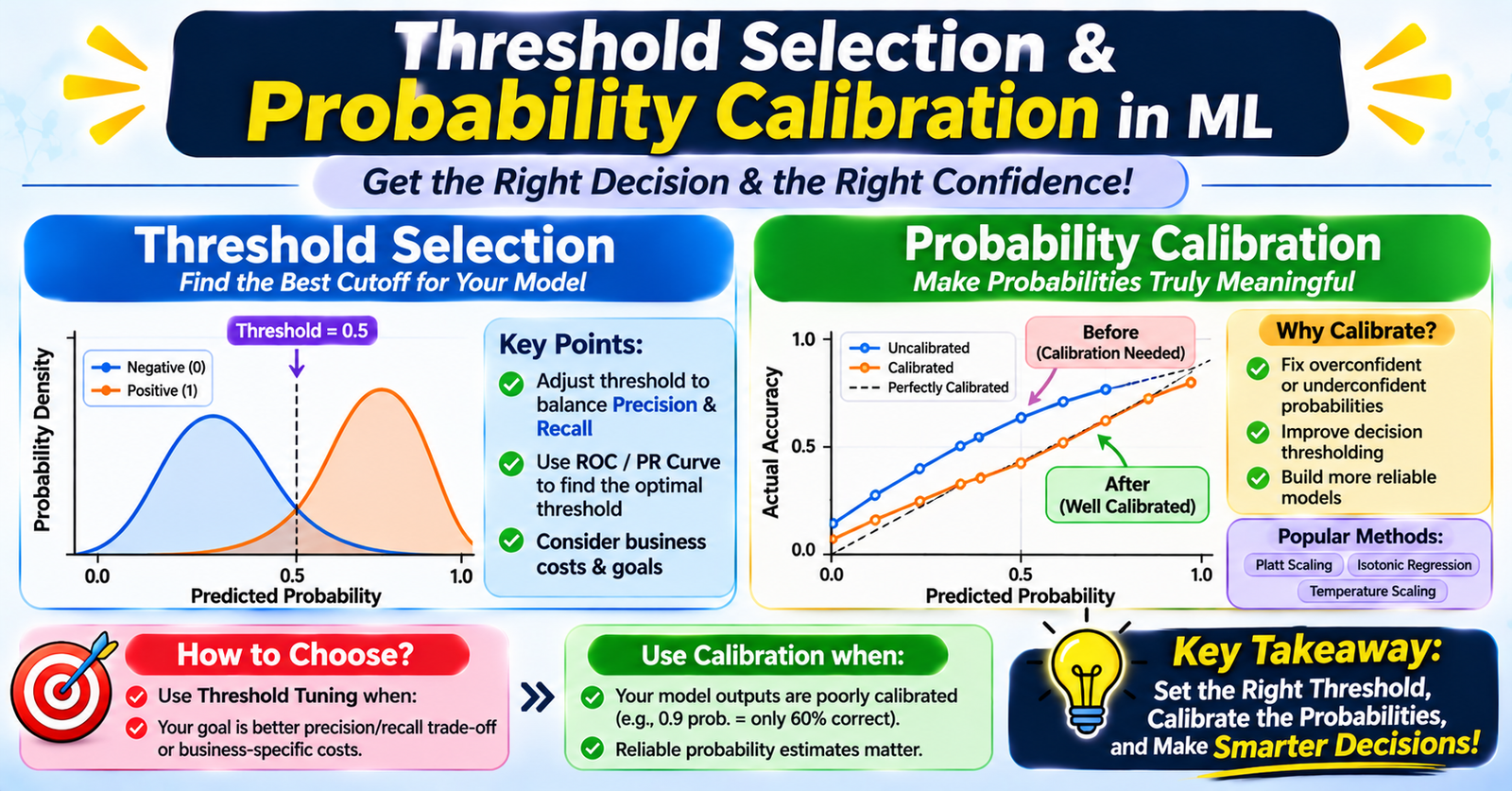
In standard classification tutorials, algorithms output a float between 0.0 and 1.0, and by default, anything $\ge 0.5$ is classified as positive.
In real-world production systems, the default 0.5 threshold is almost never optimal, and the predicted numbers are rarely true probabilities.
A model might output 0.92, but out of 100 predictions with that score, only 65 may actually be positive. If you deploy such a model into high-stakes environments—like credit lending, fraud detection, or clinical triage—you risk severe financial or operational damage.
Building dependable decision systems requires two complementary steps: Probability Calibration (ensuring the score reflects true empirical risk) and Threshold Selection (picking the exact cutoff that maximizes real-world utility).
1. Why Raw Model Outputs Are Not Probabilities
Most classification algorithms do not naturally produce well-calibrated posterior probabilities $P(Y=1 \mid X)$:
- Support Vector Machines (SVMs): Output signed uncalibrated distances to the separating hyperplane ($[-\infty, +\infty]$). Passing these through a logistic sigmoid produces distorted probabilities.
- Tree-Based Ensembles (Random Forests, XGBoost, LightGBM): Pushed toward extreme or mid-range probability spikes. Random forest predictions are averages of binary leaf outputs, which pushes extreme probabilities toward the center. Gradient boosted trees optimize ranking loss rather than likelihood, causing severe probability distortions.
- Deep Neural Networks: Modern over-parameterized neural networks often suffer from extreme overconfidence. A model may output $0.999$ confidence on an ambiguous edge-case simply because cross-entropy loss continues driving logit magnitudes higher during training.
Definition of a Calibrated Model: A model is calibrated if, among instances assigned a predicted probability of $p$, the true fraction of positive instances is exactly $p$. For example, among all samples predicted with probability $0.80$, exactly $80\%$ must be true positives.
2. Diagnosing Calibration: Reliability Diagrams & Brier Score
Before attempting any fix, evaluate your model's calibration on a held-out validation set.
Reliability Diagram (Calibration Curve)
- Bin predicted probabilities into equal buckets (e.g., $[0.0–0.1], [0.1–0.2], \dots, [0.9–1.0]$).
- For each bin, calculate the average predicted probability (x-axis) and the fraction of true positive labels (y-axis).
- A perfectly calibrated model forms an exact diagonal line $y = x$.
Fraction of Positives
      ^
  1.0 |                                 / (Perfect Calibration)
      |                              .-'
      |                           .-'
      |                        .-'  * (Underconfident)
      |                     .-'   *
      |                  .-'    *
      |               .-'     *
      |            .-' *  * (Overconfident)
      |         .-'
  0.0 +--------+------------------------>
     0.0                               1.0
             Mean Predicted Probability