Decision trees are among the most intuitive and interpretable models in machine learning. Instead of computing a linear boundary or mapping inputs into high-dimensional latent space, a decision tree asks a sequence of hierarchical "if-else" questions to segment data into homogeneous regions.
The critical question in building a decision tree is: how does the algorithm know which feature to split on, and at what specific cutoff?
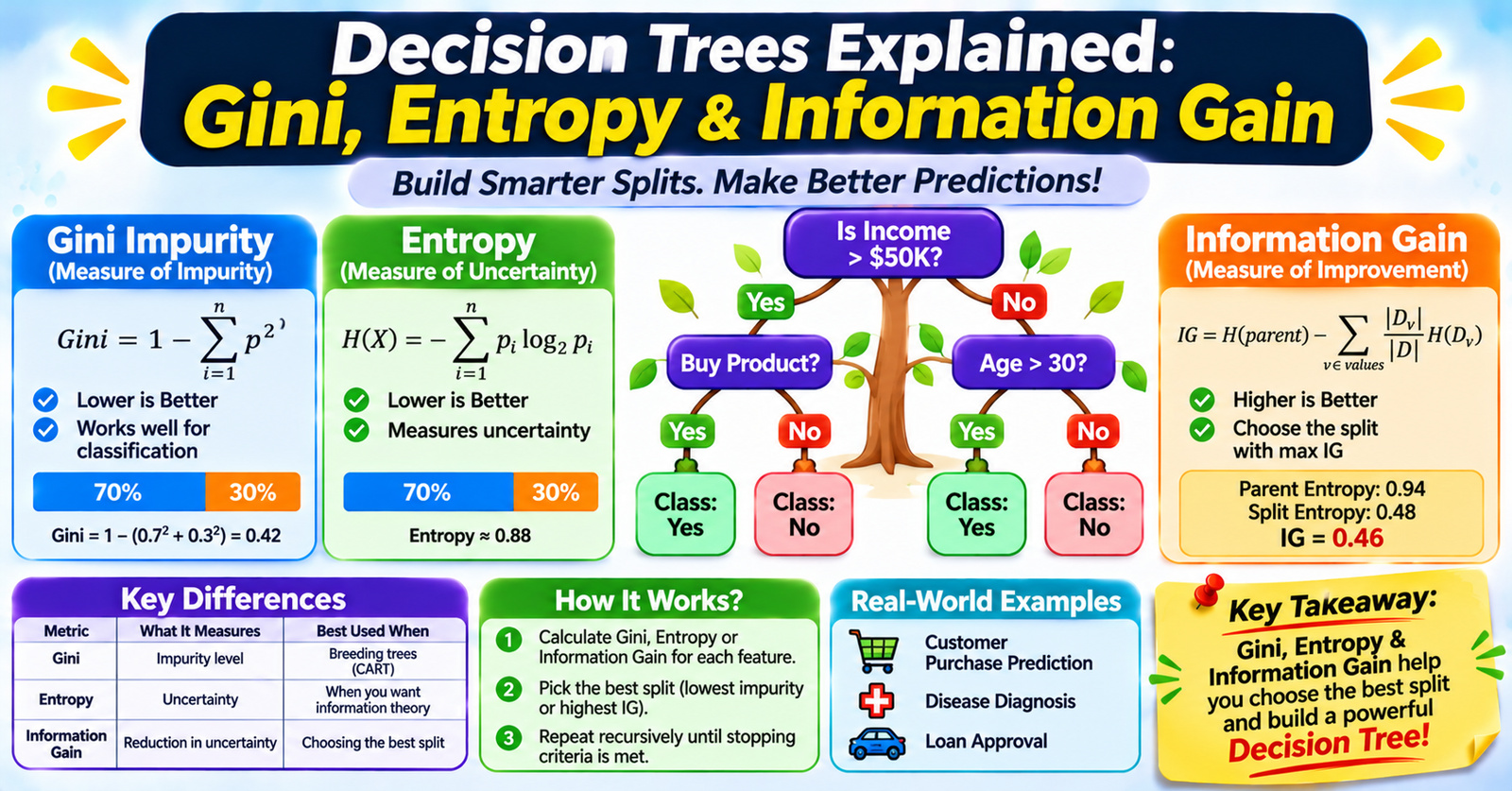
To make this decision, tree algorithms evaluate mathematical split criteria that quantify dataset uncertainty and impurity. The three primary metrics are Entropy, Information Gain, and Gini Impurity.
1. Understanding Node Impurity
A decision tree strives to partition mixed data points into subsets where instances belong overwhelmingly to a single target class.
- Pure Node: Every sample in the node belongs to the exact same class (e.g., 50 spam emails, 0 legitimate emails). Impurity is zero.
- Impure Node: Samples are evenly mixed across classes (e.g., 25 spam emails, 25 legitimate emails). Impurity is maximized.
At each step, the tree tests all candidate features and split thresholds, choosing the one that causes the largest drop in impurity from the parent node to the resulting child nodes.
2. Entropy: Measuring Uncertainty
Rooted in Claude Shannon’s Information Theory, Entropy measures the average amount of unpredictability or disorder within a distribution.
Mathematical Formula
For a node with $C$ target classes where $p_i$ is the probability (proportion) of instances belonging to class $i$:
$$H(S) = -\sum_{i=1}^{C} p_i \log_2(p_i)$$
(By convention, if $p_i = 0$, $0 \cdot \log_2(0) = 0$.)
Boundary Behavior (Binary Classification)
- Minimum ($H = 0$): All samples belong to one class ($p_1 = 1, p_2 = 0$). There is zero uncertainty.
- Maximum ($H = 1.0$): Samples are split equally ($p_1 = 0.5, p_2 = 0.5$). Uncertainty is complete.
3. Information Gain: Evaluating the Split
Entropy alone only describes a single node. Information Gain (IG) measures how much entropy decreases after partitioning a parent dataset $S$ into $K$ subsets based on a feature test $A$:
$$\text{IG}(S, A) = H(S) - \sum_{v=1}^{K} \frac{|S_v|}{|S|} H(S_v)$$
Where:
- $H(S)$ is the entropy of the parent node.
- $|S_v| / |S|$ is the proportion of total samples routed into child branch $v$.
- $H(S_v)$ is the entropy of child node $v$.
The Greedy Choice
Algorithms like ID3 and C4.5 calculate the Information Gain for every possible feature and select the split that maximizes $\text{IG}(S, A)$.
Caution with High-Cardinality Features: Pure Information Gain is inherently biased toward features with many unique values (e.g., User IDs or Transaction Numbers). Splitting on User ID produces trivial child nodes of size 1 with zero entropy, yielding massive Information Gain while failing completely to generalize. The Gain Ratio (used in C4.5) normalizes this bias using intrinsic split information.
4. Gini Impurity: The Computationally Efficient Default
Gini Impurity measures the likelihood that a randomly chosen element from a node would be incorrectly labeled if it were labeled randomly according to the class distribution within that node.
It is the standard split criterion used by the CART (Classification and Regression Trees) algorithm, which powers implementations in scikit-learn.
Mathematical Formula
$$Gini(S) = 1 - \sum_{i=1}^{C} p_i^2$$
Boundary Behavior (Binary Classification)
- Minimum ($Gini = 0$): The node is pure ($1 - (1^2 + 0^2) = 0$).
- Maximum ($Gini = 0.5$): The classes are equally distributed ($1 - (0.5^2 + 0.5^2) = 0.5$).
To evaluate a split using Gini, CART calculates the Gini Gain (reduction in weighted Gini impurity):
$$\Delta Gini = Gini(S) - \sum_{v=1}^{K} \frac{|S_v|}{|S|} Gini(S_v)$$
5. Gini Impurity vs. Entropy
| Metric | Gini Impurity | Entropy / Information Gain |
|---|---|---|
| Mathematical Range | $0.0$ to $0.5$ (binary) | $0.0$ to $1.0$ (binary, base-2 log) |
| Computation Speed | Faster (involves basic squaring) | Slower (requires logarithmic calculations) |
| Algorithmic Origin | CART | ID3, C4.5 |
| Practical Impact | Produces nearly identical tree structures in 98% of real-world use cases | Occasionally produces slightly more balanced tree depths |
| Industry Default | Standard default in scikit-learn (criterion='gini') | Optional hyperparameter (criterion='entropy') |
Because Gini avoids computing logarithms, it trains noticeably faster on large datasets while delivering virtually identical predictive performance.
6. How Regression Trees Split Data
When target values are continuous numbers rather than discrete classes, Gini and Entropy cannot be used. Instead, regression trees evaluate splits by minimizing Variance or Mean Squared Error (MSE):
$$\text{MSE}(S) = \frac{1}{|S|} \sum_{i \in S} (y_i - \bar{y}_S)^2$$
Where $\bar{y}_S$ is the average target value of all samples in node $S$. A split is chosen to maximize the reduction in total sum of squared errors between parent and child nodes.
7. Preventing Overfitting: Pruning and Constraints
Because a decision tree can continually split nodes until every single sample sits in its own leaf, unconstrained trees almost always suffer from severe high variance and overfitting.
To keep trees generalizable, apply hyperparameter constraints and pruning:
max_depth: Restricts how many vertical levels the tree can build.min_samples_split: Minimum number of samples a node must contain before an additional split is attempted.min_samples_leaf: Guarantees that every leaf contains at least $N$ samples, preventing the model from isolating individual outliers.- Cost-Complexity Pruning ($\alpha$ pruning): Trains a large unconstrained tree and subsequently prunes back weak branches that contribute minimal loss reduction relative to tree size complexity penalties.