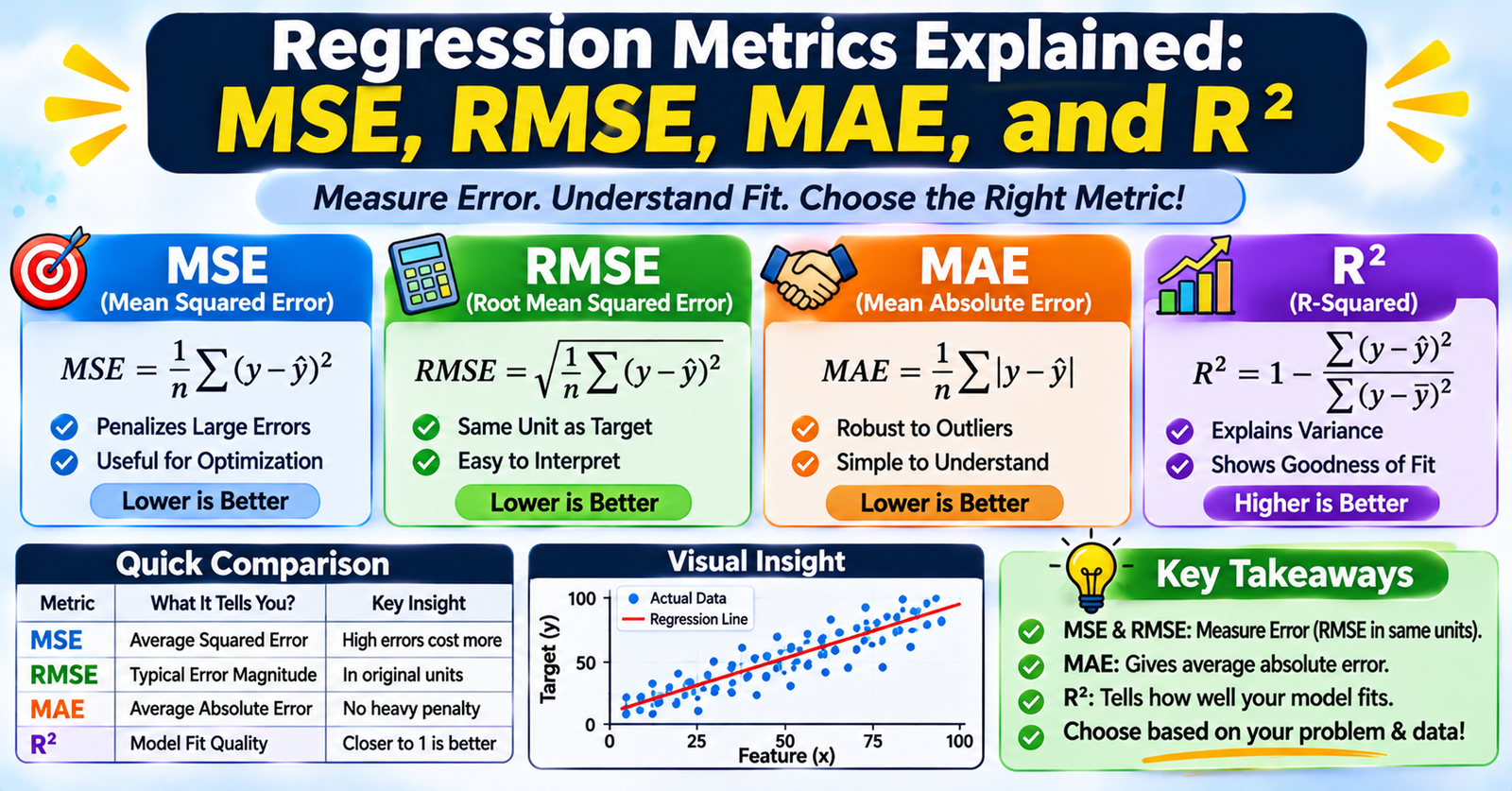
When building a regression model to predict continuous values—such as house prices, stock prices, or server latency—you cannot evaluate performance using classification accuracy. Instead, you must measure the distance between the model's predictions ($\hat{y}_i$) and the actual ground-truth values ($y_i$).
The four most widely used evaluation metrics are Mean Squared Error (MSE), Root Mean Squared Error (RMSE), Mean Absolute Error (MAE), and the Coefficient of Determination ($R^2$).
Each metric penalizes errors differently and serves distinct diagnostic purposes. Choosing the wrong one can give you an unrealistic view of how your model behaves in production.
1. Mean Absolute Error (MAE)
Mean Absolute Error calculates the average of the absolute differences between predictions and actual targets.
$$\text{MAE} = \frac{1}{n} \sum_{i=1}^{n} |y_i - \hat{y}_i|$$
Key Characteristics
- Identical Units: MAE is expressed in the exact same physical units as the target variable (e.g., dollars, seconds, kilograms), making it intuitive to explain to business stakeholders.
- Linear Penalty: Every error is weighted proportionally to its absolute magnitude. An error of 10 is penalized exactly twice as much as an error of 5.
- Robust to Outliers: Because errors are not squared, rare extreme anomalies or noisy measurement spikes do not disproportionately distort the overall metric.
When to Use MAE
- Your dataset contains known outliers or noise that you do not want dominating your model evaluation.
- You need an easily interpretable "average error" for non-technical stakeholders.
2. Mean Squared Error (MSE)
Mean Squared Error calculates the average of the squared differences between predictions and actual targets.
$$\text{MSE} = \frac{1}{n} \sum_{i=1}^{n} (y_i - \hat{y}_i)^2$$
Key Characteristics
- Quadratic Penalty: Because errors are squared before averaging, large errors are penalized far more severely than small ones. An error of 10 contributes $10^2 = 100$ to the loss, whereas an error of 5 contributes only $5^2 = 25$ (a $4\times$ penalty).
- Unit Distortion: The output units are squared (e.g., $\text{dollars}^2$ or $\text{seconds}^2$), which makes direct real-world interpretation difficult.
- Optimization Friendly: MSE is smoothly differentiable everywhere (unlike MAE, which has an undefined derivative at zero), making it a popular internal loss function for gradient descent.
When to Use MSE
- You want a mathematically smooth loss function during gradient-based training.
- Large errors are dangerous and must be penalized aggressively.
3. Root Mean Squared Error (RMSE)
Root Mean Squared Error is simply the square root of MSE, bringing the error metric back into the original units of the target variable.
$$\text{RMSE} = \sqrt{\frac{1}{n} \sum_{i=1}^{n} (y_i - \hat{y}_i)^2}$$
Key Characteristics
- Original Units Restored: Like MAE, RMSE is expressed in the original units of the target variable.
- Sensitivity to Large Errors: Unlike MAE, RMSE retains the heavy quadratic penalty on large errors before taking the root. Because of this, $\text{RMSE} \ge \text{MAE}$ is always true.
- The Gap Indicator ($\text{RMSE} - \text{MAE}$): A large gap between RMSE and MAE indicates that the model is making a few unusually large errors or that outliers are present in the dataset.
When to Use RMSE
- Large errors are significantly more costly than small errors, and you still need the metric in interpretable target units.
- Standard default for competitive benchmarking and engineering evaluations.
4. R-Squared ($R^2$ Score): Coefficient of Determination
While MAE and RMSE measure absolute scale-dependent error, $R^2$ provides a relative, scale-independent score indicating how much variance the model explains compared to a trivial baseline.
$$R^2 = 1 - \frac{\text{SS}{\text{res}}}{\text{SS}{\text{tot}}} = 1 - \frac{\sum (y_i - \hat{y}_i)^2}{\sum (y_i - \bar{y})^2}$$
Where:
- $\text{SS}_{\text{res}}$: Residual Sum of Squares (errors from your model).
- $\text{SS}_{\text{tot}}$: Total Sum of Squares (errors from a baseline model that simply predicts the mean $\bar{y}$ for every sample).
Interpreting $R^2$ Values
- $R^2 = 1.0$: Perfect model; explains 100% of the variance in the target.
- $R^2 = 0.0$: The model performs no better than simply predicting the mean $\bar{y}$ for every sample.
- $R^2 < 0.0$: The model performs worse than the baseline mean, indicating severe misfitting or improper cross-validation splits.
Caution with $R^2$: Adding more input features will almost always increase $R^2$, even if the features are random noise. To account for feature bloat, always check Adjusted $R^2$ in multiple linear regression.
Comparison Matrix
| Metric | Formula | Output Units | Outlier Sensitivity | Best Used For |
|---|---|---|---|---|
| MAE | $\frac{1}{n}\sum \ | y - \hat{y}\ | $ | Original units |
| MSE | $\frac{1}{n}\sum (y - \hat{y})^2$ | Squared units ($\text{units}^2$) | Very High | Optimization loss functions during gradient descent |
| RMSE | $\sqrt{\text{MSE}}$ | Original units | High | Catching severe deviations while retaining original units |
| $R^2$ | $1 - \frac{\text{SS}{\text{res}}}{\text{SS}{\text{tot}}}$ | Dimensionless ($-\infty$ to $1.0$) | High (derived from squared error) | Cross-dataset comparison and variance explanation |
Practical Metric Selection Guide
To select the right metric for your regression problem:
- Are large errors disproportionately worse than small ones? - Yes: Use RMSE as your primary reporting metric and MSE as your loss function. - No: Use MAE to prevent rare anomalies from skewing your evaluation.
- Do you need to compare model performance across two datasets with completely different price/unit scales? - Use $R^2$ (or Adjusted $R^2$) because it normalizes performance relative to baseline variance.
- Want a quick diagnostic check for outliers? - Compute both RMSE and MAE: if $\text{RMSE} \gg \text{MAE}$, examine your largest prediction residuals to locate extreme outliers.