When working with structured, tabular datasets, ensemble tree algorithms consistently outperform deep neural networks in training speed, interpretability, and predictive accuracy.
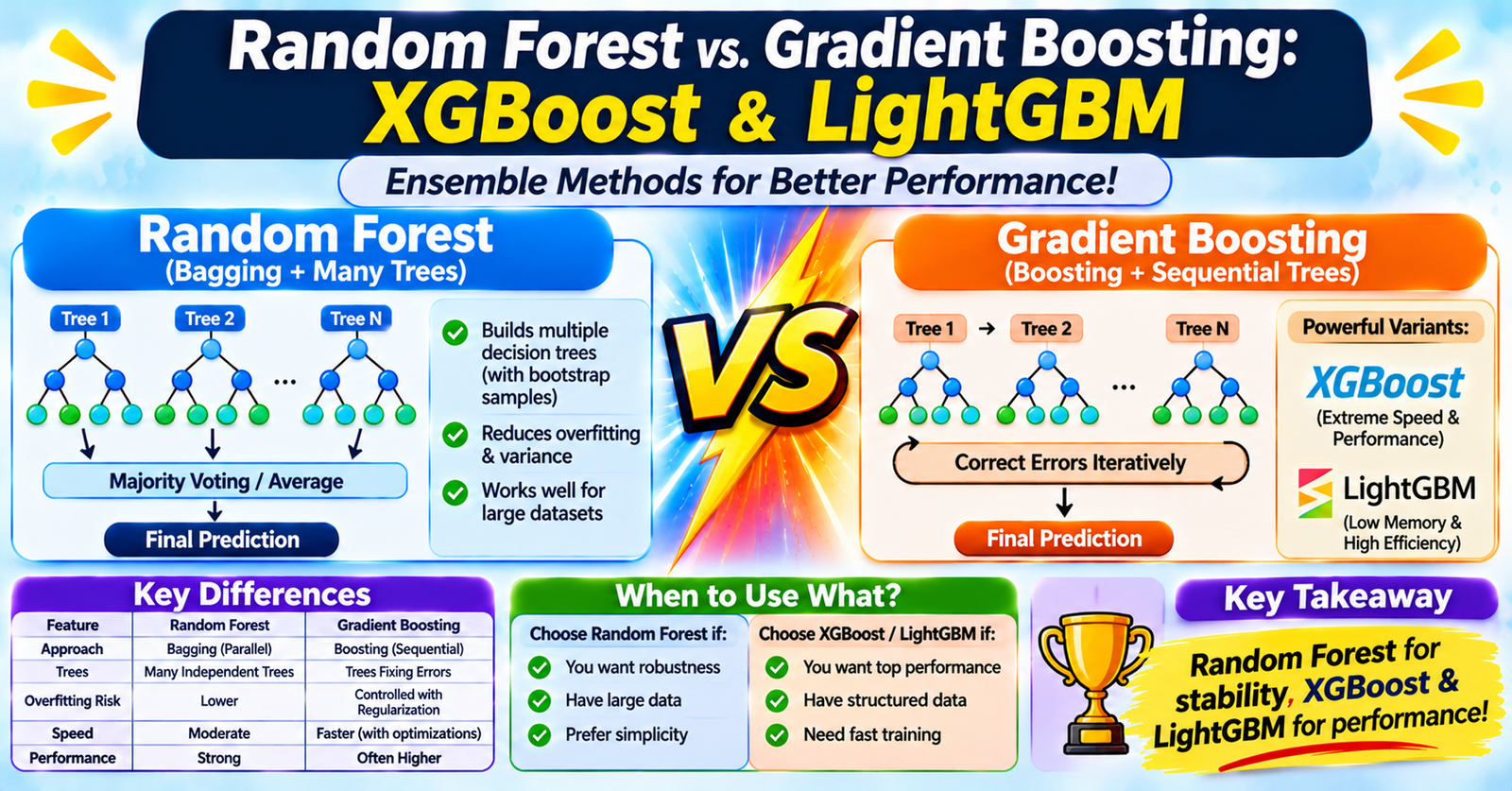
The two dominant paradigms in tree-based machine learning are Bagging (championed by Random Forests) and Boosting (dominated by XGBoost and LightGBM).
While both build collections of decision trees to make predictions, they construct those trees using opposing learning philosophies. Choosing the wrong paradigm can lead to excessive training latency, severe overfitting, or suboptimal accuracy.
1. The Core Philosophy: Bagging vs. Boosting
A single unconstrained decision tree suffers from high variance: it easily overfits noisy training data. Ensembles solve this by combining many individual trees into a unified model.
| Dimension | Random Forest (Bagging) | Gradient Boosting (Boosting) |
|---|---|---|
| Ensemble Paradigm | Bootstrap Aggregation (Bagging) | Sequential Additive Modeling (Boosting) |
| Tree Construction | Completely independent and in parallel | Sequential; each tree depends on prior trees |
| Individual Base Learner | Deep, low-bias, high-variance trees | Shallow, high-bias, weak learners ("stumps") |
| Error Reduction Focus | Variance reduction via averaging | Bias reduction via residual correction |
| Aggregation Method | Simple majority voting or equal averaging | Weighted summation scaled by learning rate $\eta$ |
2. Random Forests: Parallel Averaging
A Random Forest trains hundreds of diverse, deep decision trees independently and averages their predictions.
How Random Forest Works
- Bootstrap Sampling (Bagging): Each tree trains on an independent random sample of size $N$ drawn with replacement from the original training dataset (leaving ~36.8% of data as out-of-bag validation samples).
- Feature Randomization: At each node split, the algorithm evaluates only a random subset of features (typically $\sqrt{p}$ features) rather than all $p$ available predictors. This prevents dominant features from making every tree identical.
- Parallel Execution: Because every tree is completely independent of the others, all trees can be trained simultaneously across multiple CPU cores.
- Final Prediction: Predictions are averaged across all trees:
$$\hat{y} = \frac{1}{B} \sum_{b=1}^{B} T_b(x)$$
Strengths & Weaknesses
- Strengths: Nearly impossible to overfit by simply adding more trees; highly robust out-of-the-box with minimal hyperparameter tuning; handles noisy data and outliers gracefully.
- Weaknesses: Large memory footprint; cannot extrapolate trends beyond the minimum and maximum values seen during training; higher inference latency compared to shallow boosted models.
3. Gradient Boosting: Sequential Residual Correction
Instead of training trees independently, Gradient Boosting builds trees sequentially in a forward stagewise manner. Each new tree is explicitly trained to predict and correct the pseudo-residuals (errors) made by all previous trees combined.
The Boosting Mechanism
- Begin with an initial constant base prediction $F_0(x)$ (e.g., the average target value $\bar{y}$ for regression or log-odds for classification).
- For iteration $m = 1$ to $M$: - Calculate the negative gradient of the loss function with respect to the current predictions (the residual errors): $$r_{im} = -\left[ \frac{\partial L(y_i, F(x_i))}{\partial F(x_i)} \right]{F(x) = F{m-1}(x)}$$ - Train a shallow decision tree $h_m(x)$ to predict these residual errors $r_{im}$. - Update the ensemble by adding the new tree, scaled by a shrinkage factor or learning rate ($\eta \in (0, 1]$): $$F_m(x) = F_{m-1}(x) + \eta \cdot h_m(x)$$
By setting $\eta$ small (e.g., $0.01$–$0.1$), the algorithm takes conservative, incremental steps toward the global error minimum without overshooting.
4. XGBoost vs. LightGBM: Modern Implementations
While classic Gradient Boosted Machines (GBM) were computationally slow, XGBoost and LightGBM introduced algorithmic breakthroughs that revolutionized competitive data science.
XGBoost (Extreme Gradient Boosting)
- Second-Order Approximations: Uses both first-order gradients ($g_i$) and second-order Hessians ($h_i$) via Taylor expansion, providing a much more accurate loss landscape approximation.
- Built-in Regularization: Penalizes tree complexity directly in the loss function via $L_1$ ($\alpha$) and $L_2$ ($\lambda$) weight penalties on leaf scores: $$\Omega(f) = \gamma T + \frac{1}{2} \lambda \sum_{j=1}^{T} w_j^2$$
- Pre-Sorted & Histogram Exact Splitting: Evaluates split candidates across sorted feature distributions, guaranteeing high precision on numerical boundaries.
LightGBM (Light Gradient Boosting Machine)
Developed by Microsoft to address the memory and scalability limitations of XGBoost on massive datasets:
- Histogram-Based Binning: Continuous floating-point features are bucketed into discrete integer bins (typically 256 bins), reducing memory usage by up to $80\%$ and accelerating split computation.
- GOSS (Gradient-based One-Side Sampling): Keeps all instances with large gradients (under-trained points) and performs random sampling on instances with small gradients (well-trained points), dramatically cutting training iterations without sacrificing accuracy.
- EFB (Exclusive Feature Bundling): Mutually exclusive sparse features (such as one-hot encoded categories) are bundled into single dense features.
- Leaf-Wise (Best-First) Tree Growth: Unlike XGBoost's default level-wise (balanced) tree expansion, LightGBM splits the single leaf that yields the largest loss reduction, producing deeper, asymmetrical trees with lower loss.
Level-Wise Growth (XGBoost Default)             Leaf-Wise Growth (LightGBM)
              O                                              O
            /   \                                          /   \
           O     O                                        O     O
          / \   / \                                            / \
         O   O O   O                                          O   O
   (Splits all leaves at depth d)                                / \
                                                                O   O
                                                  (Splits highest-gain leaf only)