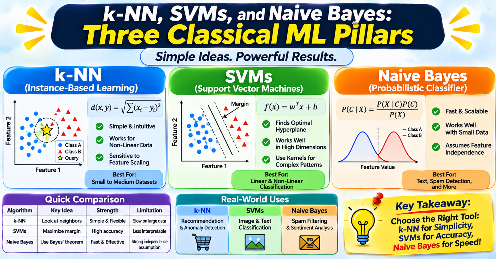
Before the widespread adoption of deep neural networks and gradient-boosted decision trees, classical machine learning relied on a distinct trio of foundational algorithms: k-Nearest Neighbors (k-NN), Support Vector Machines (SVMs), and Naive Bayes.
Each algorithm represents a completely different philosophy of learning from data:
- k-NN memorizes local geometry without training an explicit parametric model (instance-based learning).
- SVMs optimize geometric margins and use mathematical transformations to separate complex spaces (margin-based learning).
- Naive Bayes applies statistical probability and Bayes' Theorem under simplifying independence assumptions (probabilistic learning).
Understanding how these three paradigms work—and when their fundamental assumptions hold or fail—is essential for any machine learning engineer.
1. k-Nearest Neighbors (k-NN): Instance-Based Learning
k-NN is a non-parametric, lazy learning algorithm. It does not learn an explicit discriminative function or adjust internal mathematical weights during a training phase. Instead, it stores the entire training dataset in memory and defers all computation until inference time.
How k-NN Works
When given an unseen query point $x_q$:
- Compute Distance: Measure the geometric distance between $x_q$ and every stored point in the training dataset using a distance metric: - Euclidean Distance ($L_2$): $d(x, z) = \sqrt{\sum_{i=1}^p (x_i - z_i)^2}$ - Manhattan Distance ($L_1$): $d(x, z) = \sum_{i=1}^p \vert{}x_i - z_i\vert{}$ - Minkowski Distance ($L_p$): Generalization parameterizable by exponent $p$.
- Find the Neighbors: Select the $k$ closest training points.
- Aggregate: - Classification: Assign the majority label among the $k$ neighbors (or distance-weighted vote). - Regression: Compute the mean (or distance-weighted average) of the $k$ neighbor targets.
The Role of $k$ (Bias vs. Variance)
- $k = 1$: Extreme flexibility. The decision boundary wraps tightly around every individual training point, creating a complex boundary vulnerable to noise and outliers (high variance / overfitting).
- Large $k$ (e.g., $k = 100$): Smooths the decision boundary by averaging across broad neighborhoods. If $k = N$ (entire dataset size), the model simply predicts the majority class everywhere (high bias / underfitting).
Critical Pitfalls: Scaling and Dimensionality
- Feature Scale Sensitivity: Because distances are measured across coordinate axes, a feature with values in the thousands (e.g., annual income) will completely dominate a feature with values between 0 and 1 (e.g., age ratio). Features must always be normalized or standardized before running k-NN.
- The Curse of Dimensionality: As feature dimensions ($p$) grow, the volume of feature space expands exponentially. In 100+ dimensions, data points become equidistant from one another, rendering Euclidean distance uninformative.
- Inference Latency: Because prediction requires scanning and computing distances across $N$ training samples, inference scales at $\mathcal{O}(N \cdot p)$ unless accelerated by tree indexes like KD-Trees or Ball Trees.
2. Support Vector Machines (SVM) & The Kernel Trick
Support Vector Machines find an optimal boundary that separates classes while maximizing the geometric margin—the physical distance between the boundary and the closest data points from each class.
       Class A                     Margin
          o              /          <-->
       o     o          /            |
          o   (SV) --->[o]           |
      ------------------+------------+----------------- Hyperplane: w^T x + b = 0
                       [*] <--- (SV) |
                     *      *        |
                   *    *            |
             Class B